Create a LcpFinder

Creates a LcpFinder object that can then be used by find_lcp and find_lcps to find least-cost paths (LCPs) using a Quadtree as a resistance surface.

# S4 method for Quadtree
lcp_finder(
  x,
  start_point,
  xlim = NULL,
  ylim = NULL,
  new_points = matrix(nrow = 0, ncol = 2),
  search_by_centroid = FALSE
)

Arguments

x

a Quadtree to be used as a resistance surface

start_point

two-element numeric vector (x, y) - the x and y coordinates of the starting point

xlim

two-element numeric vector (xmin, xmax) - constrains the nodes included in the network to those whose x limits fall in the range specified in xlim. If NULL the x limits of x are used

ylim

same as xlim, but for y

new_points

a two-column matrix representing point coordinates. First column contains the x-coordinates, second column contains the y-coordinates. This matrix specifies point locations to use instead of the node centroids. See 'Details' for more.

search_by_centroid

boolean; determines which cells are considered to be "in" the box specified by xlim and ylim. If FALSE (the default) any cell that overlaps with the box is included. If TRUE, a cell is only included if its centroid falls inside the box.

Value

a LcpFinder

Details

See the vignette 'quadtree-lcp' for more details and examples (i.e. run vignette("quadtree-lcp", package = "quadtree"))

To find a least-cost path, the cells are treated as points - by default, the cell centroids are used. This results in some degree of error, especially for large cells. The new_points parameter can be used to specify the points used to represent the cells - this is particularly useful for specifying the points to be used for the start and end cells. Each point in the matrix will be used as the point for the cell it falls in (if two points fall in the same cell, the first point is used). Note that this raises the possibility that a straight line between neighboring cells may pass through other cells as well, which complicates the calculation of the edge cost. To mitigate this, when a straight line between neighboring cells passes through a different cell, the path is adjusted so that it actually consists of two segments - the start point to the "corner point" where the two cells meet, and then from that point to the end point. See the "quadtree-lcp" vignette for a graphical example of this situation.

An LcpFinder saves state, so once the LCP tree is calculated, individual LCPs can be retrieved without further computation. This makes it efficient at calculating multiple LCPs from a single starting point. However, in the case where only a single LCP is needed, find_lcp() offers an interface for finding an LCP without needing to use lcp_finder() to create the LcpFinder object first.

See also

find_lcp() returns the LCP between the start point and another point. find_lcps() finds all LCPs whose cost-distance is less than some value. summarize_lcps() outputs a summary matrix of all LCPs that have been calculated so far. points() and lines() can be used to plot a LcpFinder.

Examples

####### NOTE #######
# see the "quadtree-lcp" vignette for more details and examples:
# vignette("quadtree-lcp", package = "quadtree")
####################

library(quadtree)

habitat <- terra::rast(system.file("extdata", "habitat.tif", package="quadtree"))
qt <- quadtree(habitat, split_threshold = .1, adj_type = "expand")

# find the LCP between two points
start_pt <- c(6989, 34007)
end_pt <- c(33015, 38162)

# create the LCP finder object and find the LCP
lcpf <- lcp_finder(qt, start_pt)
path <- find_lcp(lcpf, end_pt)

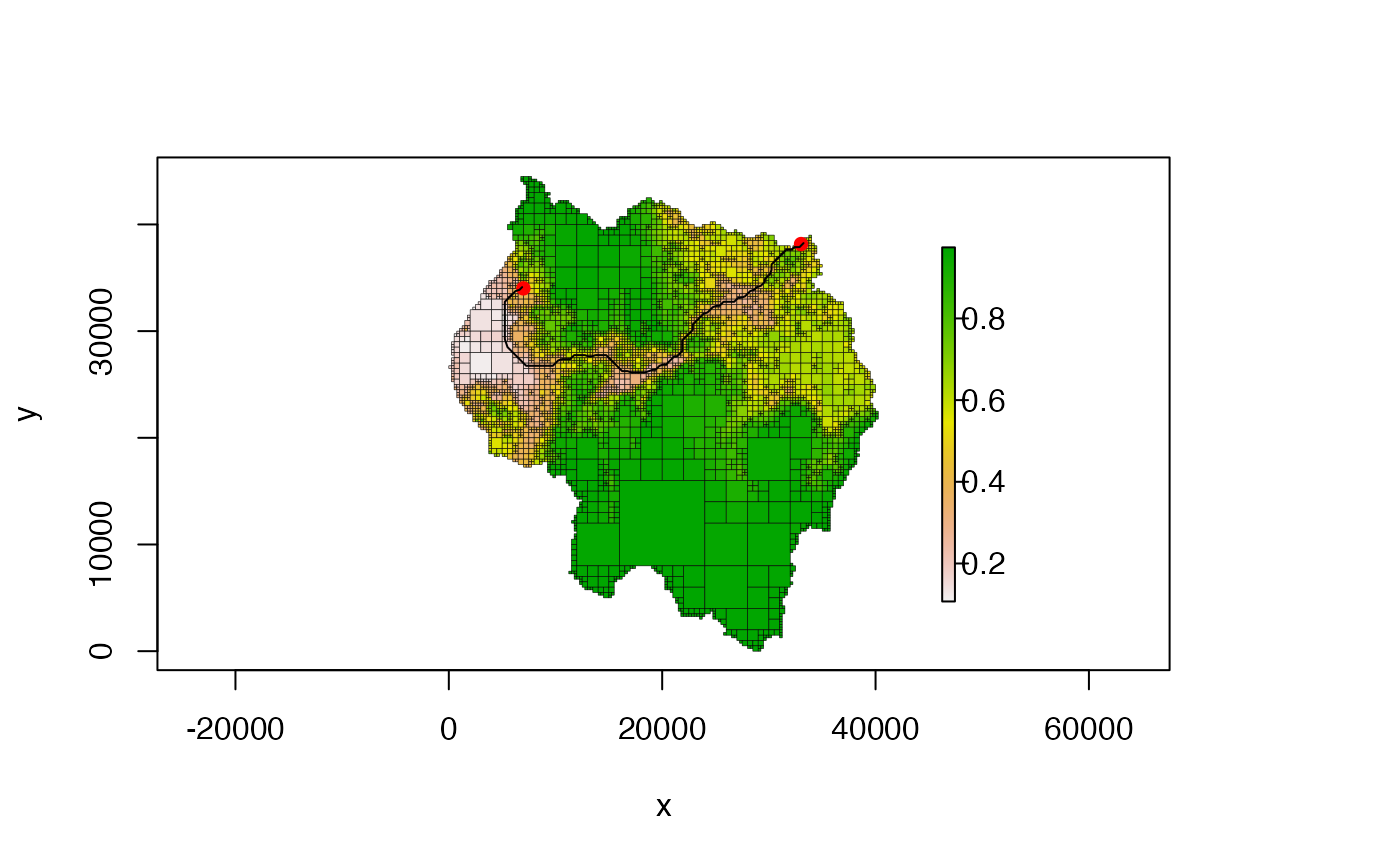
# plot the LCP
plot(qt, crop = TRUE, na_col = NULL, border_lwd = .3)
points(rbind(start_pt, end_pt), pch = 16, col = "red")
lines(path[, 1:2], col = "black")